How to Use Mean and Mean Absolute Deviation to Compare Data: Full i-Ready Guide
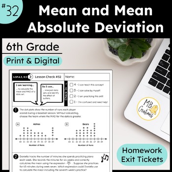
Every school week, millions of middle schoolers sit before Curriculum Associates’ adaptive i-Ready software, confronting one of seventh-grade math's most notoriously misunderstood units: comparing two data distributions using statistical measures. While calculating an average is familiar territory for most twelve-year-olds, the software shifts expectations when it introduces Mean Absolute Deviation (MAD). Suddenly, finding the middle of a data set is only half the battle.
The friction peaks when the software demands that students interpret statistical spread to draw informal comparative inferences. Frustrated parents scour forums like Reddit's r/HomeworkHelp and r/Teachers trying to decipher why two sets of test scores with identical averages tell completely different operational stories. Mastering this standard is not about memorizing digital flashcards; it is about grasping how variation reveals the true consistency of numbers.
📌 Quick Summary:
- The Method: Mean tracks the center of data, while Mean Absolute Deviation gauges statistical spread by calculating the average distance between every data point and that center.
- The Objective: In i-Ready 7th grade math, students express the distance between two sample means as a multiple of the MAD to measure visual overlap.
- The Trap: Dropping negative signs during the absolute difference calculation or miscounting values on dot plots accounts for over 70% of software error flags.
The Core Mechanics Behind Measures of Center and Variability
Statistical literacy requires understanding two distinct dimensions of a distribution: where the middle sits and how widely the surrounding values scatter. The mean serves as the primary measure of center for symmetrical data, representing an equitable balance point where the sum of positive deviations equals the sum of negative deviations.
Center alone can conceal critical realities. A student scoring 50% and 100% on two exams shares the exact same 75% mean as a student scoring 74% and 76%. This is where measures of variability step in.
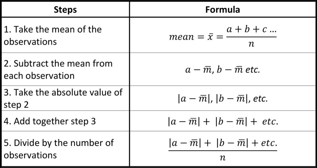
Mean Absolute Deviation (MAD) calculates the average distance of all observations from the mean. Instead of squaring differences, as seen in high school standard deviation, seventh-grade math keeps the math grounded through absolute values:
$$\text{MAD} = \frac{\sum |x - \bar{x}|}{n}$$
A lower MAD signals high consistency, clustering data points tightly around the center. A high MAD reflects wide statistical spread, showing volatile values prone to swinging far from the arithmetic baseline. When an i-Ready prompt displays side-by-side dot plots, a wider spread directly flags higher data set variability.
Step-by-Step i-Ready Lesson Walkthrough: Calculating the Mean Absolute Deviation
When navigating an i-Ready lesson walkthrough, questions typically split the calculation into three sequential steps. Skipping any of them leads straight to a diagnostic drop.
First, determine the mean of the distribution. Sum every individual value in the sample data set and divide that total by the sample size ($n$).
Second, complete the absolute difference calculation for every single number. Subtract the sample mean from each individual data point and strip away any resulting negative signs. The distance between 12 and 15 is 3; the distance between 18 and 15 is also 3. Distance in descriptive statistics cannot be negative.
Third, calculate the mean of those differences. Add every individual absolute difference together, then divide by the total count of data points.
Consider this concrete scenario from a standard problem: tracking daily peak temperatures in two coastal towns over a five-day stretch.
Town A reports temperatures of 68, 70, 72, 74, and 76 degrees. The sum equals 360. Dividing 360 by 5 yields a mean of 72 degrees. The absolute distances from 72 are:
- $|68 - 72| = 4$
- $|70 - 72| = 2$
- $|72 - 72| = 0$
- $|74 - 72| = 2$
- $|76 - 72| = 4$
Summing those five distances gives 12. Dividing 12 by 5 yields a MAD of 2.4 degrees. On average, any given day's temperature misses the weekly mean by just under two and a half degrees.
| Metric | Distribution A (Town A) | Distribution B (Town B) |
|---|---|---|
| Sample Values | 68, 70, 72, 74, 76 | 58, 64, 72, 80, 86 |
| Sum of Observations | 360 | 360 |
| Measure of Center (Mean) | 72.0°F | 72.0°F |
| Absolute Deviations | 4, 2, 0, 2, 4 | 14, 8, 0, 8, 14 |
| Sum of Deviations | 12 | 44 |
| Measure of Variability (MAD) | 2.4°F | 8.8°F |
Both locations share an identical mean of 72 degrees. Yet looking at the MAD tells the actual climatic story. Town A features a predictable microclimate, while Town B swings wildly across an 8.8-degree average deviation.
Making Informal Comparative Inferences Between Two Distributions
The ultimate hurdle on i-Ready assessments is not just finding the MAD, but using it to compare two distinct groups. Under Common Core standard 7.SP.B.3, students must formally express the difference between two centers as a multiple of a measure of variability.
When comparing two data distributions, i-Ready typically gives problems where both distributions have very similar MADs. The software then asks: "The difference between the means is approximately how many times the mean absolute deviation?"
To solve this, follow a straightforward operational formula:
$$\text{Multiple} = \frac{|\text{Mean}1 - \text{Mean}2|}{\text{MAD}}$$
Assume a middle-school athletics program tracks pull-up counts across two different homerooms:
- Group Alpha: Mean = 14 pull-ups, with a MAD of 2 pull-ups.
- Group Beta: Mean = 20 pull-ups, with a MAD of 2 pull-ups.
The difference between the two means is $20 - 14 = 6$.
Dividing that difference of 6 by the shared MAD of 2 equals 3.
The inference statement must read: The mean of Group Beta is 3 times the mean absolute deviation greater than the mean of Group Alpha.
This numerical multiple explains visual overlap on graphs. If the difference in means is tiny, say, 0.5 times the MAD, the two distributions overlap heavily on a dot plot, making the difference between groups statistically negligible. When the difference climbs to 2 or 3 times the MAD, the data clusters separate visually, proving the gap between the two cohorts is meaningful and consistent.
Common Traps in Dot Plots, Box Plots, and Software Scoring
Curriculum Associates engineers its interactive questions to catch mechanical guesses. Classroom feedback highlights three persistent failure points where students routinely forfeit progress bars.
Dot Plot Misread:
Values: 10 12 12 15
Dots: • • • •
Mistake: Entering "3 values" instead of 4 because of the stacked dot.
Result: Incorrect divisor (n=3 instead of n=4), corrupting both Mean and MAD.
The most frequent error occurs during dot plot transcription. When a dot plot displays a column of three dots above the number 8, students frequently register the number 8 once instead of entering it three distinct times. This deflates the true sample size, throwing off both the initial sum and the final denominator.
A second issue involves confusing measures of variability with measures of center when interpreting box plots. Box plots showcase the median and the Interquartile Range (IQR), not the mean and the MAD. Attempting to use the MAD formula on numbers pulled from five-number summary quartiles generates computational dead ends. Mean and MAD belong to symmetrical, distribution-wide calculations; median and IQR belong to ordinal, rank-based comparisons.
Finally, arithmetic drift ruins multi-step calculations. Students often forget to convert fractional results into clean decimals early, or they round too aggressively in the middle of calculating absolute differences. Rounding a mean from 14.333 down to 14 before subtracting can distort the final MAD by a margin large enough to trigger an error within i-Ready's automated grading engine.
Why Modern Curricula Prioritize MAD Over Standard Deviation
For decades, middle-school mathematics curricula skipped directly from simple range to high school standard deviation, forcing early learners into quadratic equations and square roots before they grasped what variability actually measured.
The shift toward emphasizing Mean Absolute Deviation in seventh-grade standards reflects modern educational learning progressions. Standard deviation artificially amplifies outlier weights by squaring differences. While essential for university research and machine learning models, squaring values confuses concrete conceptual understanding in middle school.
MAD keeps measurements strictly linear and tied to real-world units. If an urban planner studies bus arrival times, a MAD of 4 minutes directly signifies that commuters wait, on average, 4 minutes longer or shorter than the posted timetable.
Educators on platforms like Reddit's r/MathChat point out that students who grasp MAD transition far more comfortably to advanced probability and data science concepts later. They cease viewing numbers as isolated targets and begin evaluating distributions as fluid, shifting spreads.
Frequently Asked Questions (FAQ)
Q1: What is the main difference between range and Mean Absolute Deviation?
The range only measures the span between the single largest and single smallest values in a set, ignoring all numbers in between. Mean Absolute Deviation evaluates every single data point, providing a complete measurement of how the entire distribution behaves around its center.
Q2: Can the Mean Absolute Deviation ever be a negative number?
No. Because absolute values represent distance on a number line, every calculated deviation is positive or zero. Dividing a sum of positive numbers by a positive count will always yield a positive number or zero.
Q3: How do I know whether to compare data using Mean/MAD or Median/IQR?
Use Mean and MAD when the data distribution is relatively balanced, bell-shaped, and free of extreme outliers. When data is skewed or contains massive outliers that distort the average, rely on Median and Interquartile Range (IQR) instead.
Q4: Why does i-Ready ask for the difference between means as a multiple of the MAD?
This calculation prepares students for advanced statistics by introducing the concept behind effect size. Expressing the difference between two averages as a multiple of their variability confirms whether the gap between groups is meaningful or just random noise.
Mastering Data Distributions in Modern Math Classrooms
Mastering the mechanics of mean and Mean Absolute Deviation transforms raw data from an intimidating collection of numbers into an organized, readable landscape. When students stop rushing through calculations and begin identifying how individual points move around an anchor, software modules cease being an uphill battle. The real breakthrough happens when they see that numbers are not just static points on a screen, but measurements of real-world consistency. By grounding operations in precise differences and understanding how variability shapes data, students build analytical instincts that last long after the screen goes dark.